The Naive Approach
In graph databases, abstractions like vertices and edges enable us to represent entities and their relations. Applying this to the previously mentioned example, the entities Tom and Jerry can be stored as two vertices, connected by an edge representing the knows relation between them. In this case, it looks quite easy to find out whether or not Tom knows Jerry:
All we need to do is find the vertex that represents Tom, look for all the people Tom knows, and ultimately find out if Jerry is one of them. In Gremlin, such a query would look like this:
g.V().has('name', 'Tom').out('knows').has('name', 'Jerry').hasNext()
But what if Tom knows very many people? In this case, the traversal would iterate over all of them and compare each name with "Jerry" in order to search for matching neighbours. This quickly escalates when the number of adjacent vertices exceeds tens or hundreds of thousands. Let's dive in deeper and find out why!
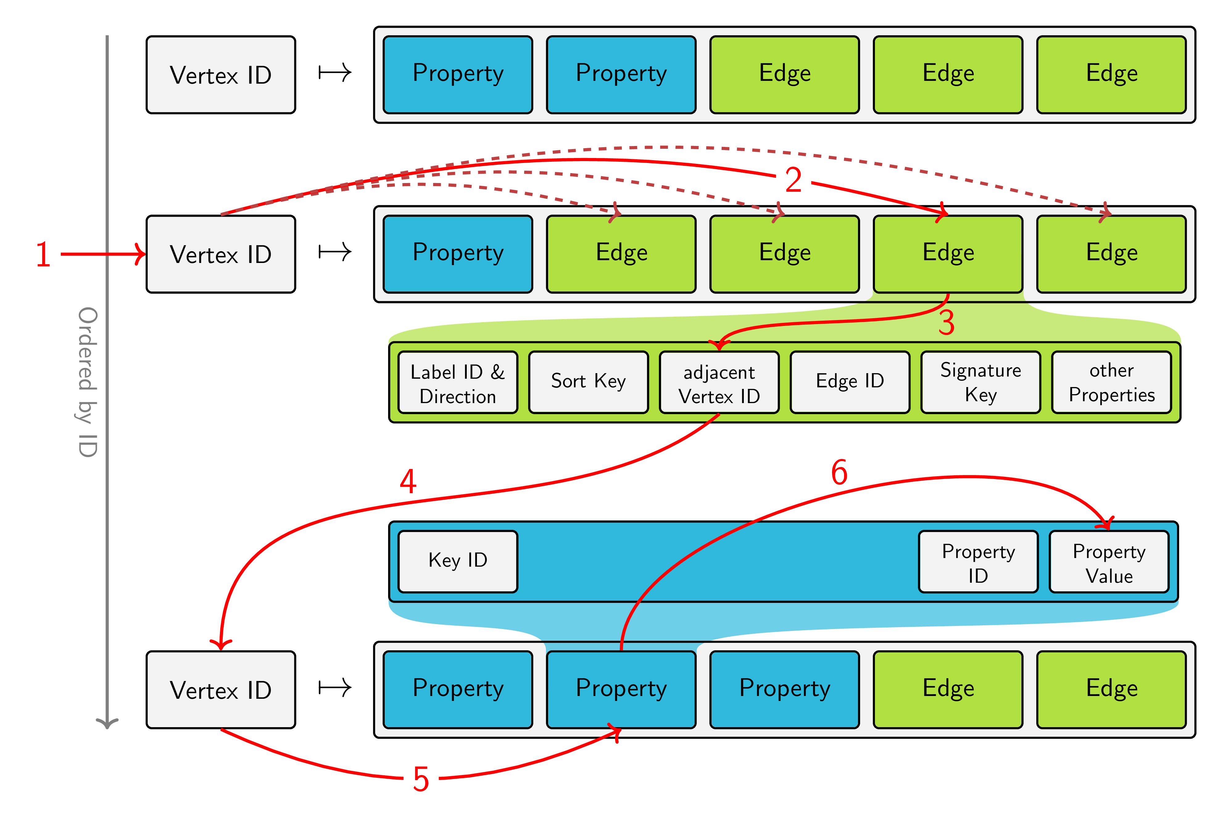
The above image shows the storage layout of JanusGraph. Vertices are stored in an ordered fashion by their ID and for each vertex, a list of its properties and adjacent edges is stored on disk. Based on this model, we can break down our query into the steps, that the underlying storage backend has to perform:
- Retrieve the vertex of Tom
- Inspect all edges adjacent to the vertex Tom (and filter them by label and direction, which is not visualized in the picture)
- Find out which vertex is located at the other end of the edge
- Jump to the storage location of this vertex
- Look at the property "name"
- Retrieve its value and check if it matches "Jerry"
What takes exceptionally long here is step number 4. Because of the storage layout, different vertices are distributed all over the available disk space. Worse, in distributed systems, they may even be located on physically different machines. And as every programmer knows, random reads are expensive. So what can we do better?
Using Indices
When analyzing the naive approach, we already made an assumption that is not trivial: We assumed it's easy to retrieve the starting point of our query, the vertex of Tom. And indeed, when utilizing JanusGraph's ability to use indices, this is an easy task. So why not use the same index to find both the vertices for Tom and Jerry first?
tom = g.V().has('name', 'Tom').next()
jerry = g.V().has('name', 'Jerry').next()
g.V(tom).out('knows').is(jerry).hasNext()
This way, we have obtained the vertex of Jerry early, which means we can skip steps 5 and 6 of our original query. Instead, what the backend now does is fetch the vertex in step 4 and compare it directly to the vertex we retreived earlier. This simplifies the query execution a little bit, but the most expensive operation still remains.
The Solution is just around the Corner
We are almost there! Taking a closer look at the storage model, we observe that the backend is already aware of Jerry's ID after executing step 3. So instead of comparing vertices directly, we can lookup Jerry's ID once in the beginning and use this ID to find matching edges after step 3. This way, the expensive step 4 is avoided, resulting in an impressive speed gain:
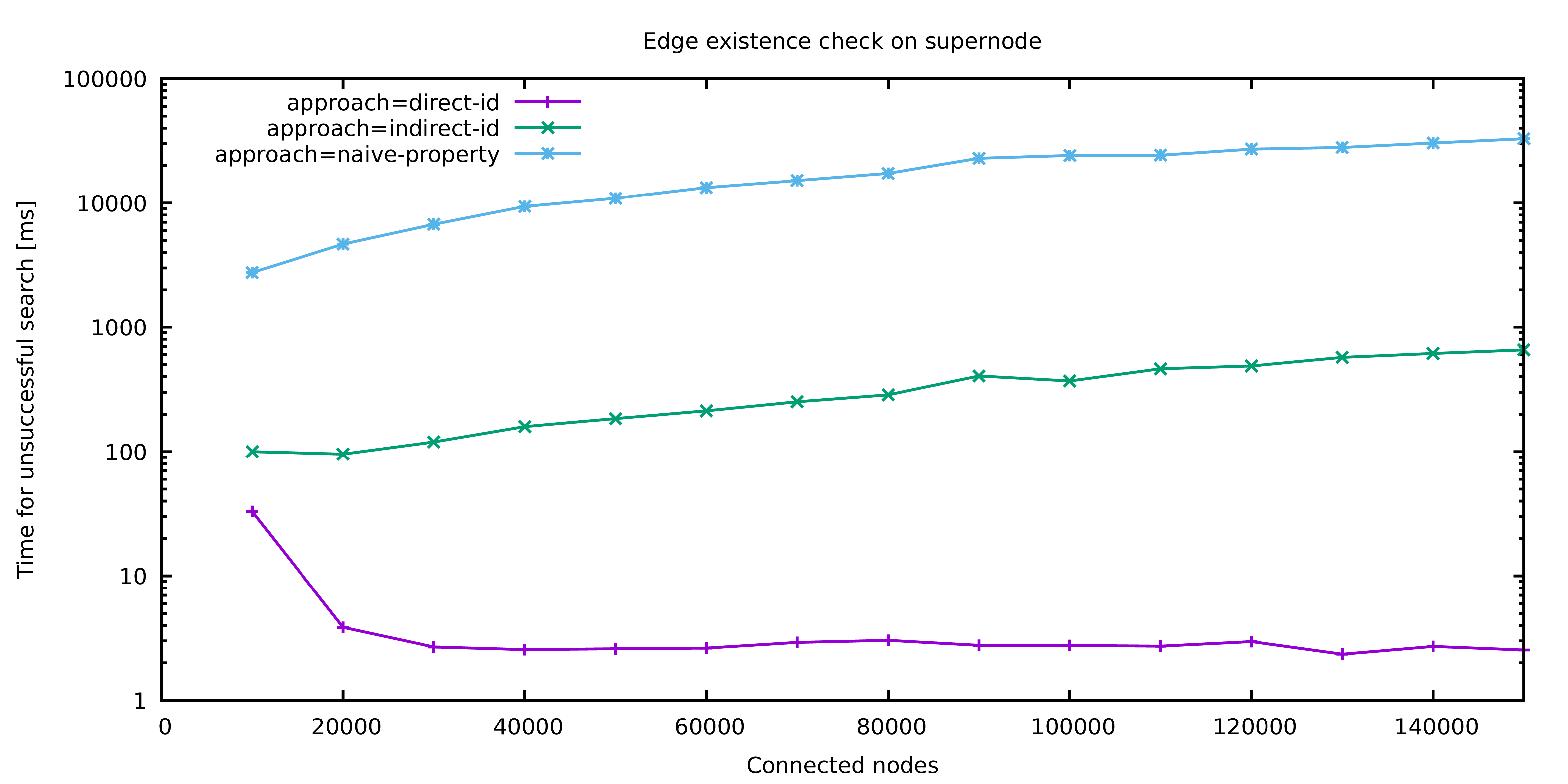
The above image shows the different approaches naive-property, indirect-id and direct-id that were presented in this article: Besides the naive approach which looks at the properties of adjacent vertices, there are two stages of optimizations. Indirect ID refers to the idea of comparing previously fetched vertices while Direct ID is the final optimization.
The difference in performance is clearly visible: While the naive approach quickly reaches a magnitude of tens of seconds, even simple improvements allow the query to finish within hundreds of milliseconds. With the most sophisticated optimization, the execution time drops to single digit milliseconds. The runs for 10.000 and 20.000 connected vertices respectively are treated as a warmup phase and the corresponding results should be used with care.
Notably, the execution time of the optimized query does not seem to depend on the number of adjacent vertices at all. This is not the case! The optimized query has a logarithmic runtime bound, because JanusGraph is clever enough to maintain an index of all edges adjacent to a vertex and use this index to answer our equality check on Jerry's vertex ID. Therefore, instead of iterating all edges, step 2 becomes a single index lookup.
Changes to JanusGraph
Utilizing our newly gained knowledge, we built multiple optimization strategies into JanusGraph which automatically rewrite queries to make use of these performance improvements. At the current state of work, the following kinds of queries are automatically optimized:
g.V(tom).outE('label').inV().is(jerry)
g.V(tom).outE('label').inV().hasId(jerry.id())
g.V(tom).out('label').is(jerry)
g.V(tom).out('label').hasId(jerry.id())
g.V(tom).out('label').filter(is(jerry))
g.V(tom).out('label').where(is(jerry))
g.V(tom).out('label').filter(hasId(jerry.id()))
g.V(tom).out('label').where(hasId(jerry.id()))
g.V(tom).outE('label').where(inV().is(jerry))
g.V(tom).outE('label').filter(inV().is(jerry))
g.V(tom).outE('label').where(inV().hasId(jerry))
g.V(tom).outE('label').filter(inV().hasId(jerry))
All of this also applies to all other valid variations of in(), out() and both() and inE()/outE() respectively. The new optimizers are available in JanusGraph version 0.5.0 or newer.